
Cluster Analysis of Insurance Customers
Imports
import pandas as pd
import numpy as np
#Plot styling
import matplotlib.pyplot as plt
import seaborn as sns; sns.set()  # for plot styling
%matplotlib inline

plt.rcParams['figure.figsize'] = (16, 9)
plt.style.use('ggplot')
df = pd.read_excel('Actual.Data.xlsx')
Exploratory Data Analysis - Takaful Dataset
df.head()
| Policy.ID | Assets | Gold.Customer | Status | Installment.Payment.Date | Next.Installment.Due.Date | Policy.Started.On | Mode | BasicPlan | Gender | ... | Customer.Age.Policy.Start | Policy.Since (Year) | Customer.Age.Current | Agent | Installment.Amount | Premium.Amount | Total.Paid | City | Single/Joint | PaymentType | |
|---|---|---|---|---|---|---|---|---|---|---|---|---|---|---|---|---|---|---|---|---|---|
| 0 | P60266 | 3 | Active | Active | 2019-05-28 00:00:00 | 2021-05-01 | 2012-05-01 | Annual | Super.Savings | M | ... | 37.0 | 9 | 45.0 | Individual | 1463119.0 | 329954.0 | 659908.0 | Karachi | Single | CHEQUE |
| 1 | P27953 | 1 | Active | Active | 2017-12-28 11:45:25 | 2021-01-01 | 2018-01-01 | Annual | Super.Savings | M | ... | 34.0 | 3 | 36.0 | Financial.Company | 1200000.0 | 300000.0 | 900000.0 | Naushera | Single | Online.Debit |
| 2 | P41583 | 1 | Active | Active | 2018-09-13 09:47:48 | 2019-10-01 | 2018-10-01 | Annual | Super.Savings | NaN | ... | 45.0 | 1 | 46.0 | Financial.Company | 750000.0 | 750000.0 | 750000.0 | Sialkot | Single | Online.Debit |
| 3 | P65843 | 1 | Active | Active | 2019-08-23 00:00:00 | 2021-10-01 | 2019-10-01 | Annual | Family.Future.Security | NaN | ... | 39.0 | 2 | 39.0 | Financial.Company | 600000.0 | 200000.0 | 400000.0 | Karachi | Single | Online.Debit |
| 4 | P40045 | 2 | Inactive | Lapsed | 2018-08-17 16:00:10 | 2019-09-01 | 2018-09-01 | Annual | Savings | F | ... | 59.0 | 1 | 60.0 | Individual | 525000.0 | 500000.0 | 500000.0 | Hyderabad | Single | CHEQUE |
5 rows × 21 columns
Data Types of columns
df.info()
<class 'pandas.core.frame.DataFrame'>
RangeIndex: 57019 entries, 0 to 57018
Data columns (total 21 columns):
Policy.ID                    57019 non-null object
Assets                       57019 non-null int64
Gold.Customer                57019 non-null object
Status                       57019 non-null object
Installment.Payment.Date     57019 non-null datetime64[ns]
Next.Installment.Due.Date    57019 non-null datetime64[ns]
Policy.Started.On            57019 non-null datetime64[ns]
Mode                         57019 non-null object
BasicPlan                    57019 non-null object
Gender                       18981 non-null object
Weight (KG)                  56968 non-null float64
Customer.Age.Policy.Start    57019 non-null float64
Policy.Since (Year)          57019 non-null int64
Customer.Age.Current         57019 non-null float64
Agent                        57019 non-null object
Installment.Amount           57019 non-null float64
Premium.Amount               57019 non-null float64
Total.Paid                   57017 non-null float64
City                         57019 non-null object
Single/Joint                 57019 non-null object
PaymentType                  57019 non-null object
dtypes: datetime64[ns](3), float64(6), int64(2), object(10)
memory usage: 9.1+ MB
Check Null Values
df.apply(lambda x: sum(x.isnull()),axis=0)
Policy.ID                        0
Assets                           0
Gold.Customer                    0
Status                           0
Installment.Payment.Date         0
Next.Installment.Due.Date        0
Policy.Started.On                0
Mode                             0
BasicPlan                        0
Gender                       38038
Weight (KG)                     51
Customer.Age.Policy.Start        0
Policy.Since (Year)              0
Customer.Age.Current             0
Agent                            0
Installment.Amount               0
Premium.Amount                   0
Total.Paid                       2
City                             0
Single/Joint                     0
PaymentType                      0
dtype: int64
df['Gender'].value_counts()
M    18344
F      637
Name: Gender, dtype: int64
df.rename(columns={'Weight (KG)': 'Weight'}, inplace=True)
Tackling Missing Values in Gender and Weight
sns.boxplot(x=df['Weight'])
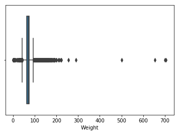
#Drop 51 null values in weight as they are very less and will not have a major impact
#df.dropna(subset=['Weight'],inplace=True)
df.apply(lambda x: sum(x.isnull()),axis=0)
Policy.ID                        0
Assets                           0
Gold.Customer                    0
Status                           0
Installment.Payment.Date         0
Next.Installment.Due.Date        0
Policy.Started.On                0
Mode                             0
BasicPlan                        0
Gender                       38038
Weight                          51
Customer.Age.Policy.Start        0
Policy.Since (Year)              0
Customer.Age.Current             0
Agent                            0
Installment.Amount               0
Premium.Amount                   0
Total.Paid                       2
City                             0
Single/Joint                     0
PaymentType                      0
dtype: int64
df.groupby('Gender')['Weight'].mean()
Gender
F    63.683533
M    70.839145
Name: Weight, dtype: float64
#Making A copy of the dataframe so that we dont lose our data while transformation
new_df = df.copy()
new_df['Gender'] = new_df['Gender'].replace(np.nan, 'X')
Replace Missing Values wrt Male and Female Averages
for i in range(len(new_df.index)):
    if new_df['Gender'].iloc[i] =='X':
        if new_df['Weight'].iloc[i] < 70.839145:
            new_df.iloc[i, new_df.columns.get_loc('Gender')] = 'F'
        else:
            new_df.iloc[i, new_df.columns.get_loc('Gender')] = 'M'
new_df.dropna(subset=['Total.Paid'],inplace=True)
#There were two Missing values in Total.Paid Column that are dropped too
#Cleaned Data
new_df.to_excel(r'E:\Semester_8\Business_Intelligence\TAKAFUL_ASSIGNMENT\Cleaned_Takaful_Dataset_Final.xlsx', index = False, header = True)
Data Visualizations
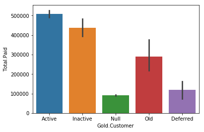
sns.barplot(x='Gold.Customer',y='Total.Paid',data=new_df)
Customer Segmentation - Installment and Premium
data = pd.read_excel('E:\Semester_8\Business_Intelligence\TAKAFUL_ASSIGNMENT\Cleaned_Takaful_Dataset_Final.xlsx')
data.info()
<class 'pandas.core.frame.DataFrame'>
RangeIndex: 57017 entries, 0 to 57016
Data columns (total 23 columns):
Policy.ID                    56567 non-null object
Assets                       56567 non-null float64
Gold.Customer                56567 non-null object
Status                       56567 non-null object
Installment.Payment.Date     56567 non-null datetime64[ns]
Next.Installment.Due.Date    56567 non-null datetime64[ns]
Policy.Started.On            56567 non-null datetime64[ns]
Mode                         56567 non-null object
BasicPlan                    56567 non-null object
Gender                       56567 non-null object
Weight                       56521 non-null float64
Customer.Age.Policy.Start    56567 non-null float64
Policy.Since (Year)          56567 non-null float64
Customer.Age.Current         56567 non-null float64
Agent                        56567 non-null object
Installment.Amount           56567 non-null float64
Installment_Amount           57017 non-null int64
Premium.Amount               56567 non-null float64
Premium_Amount               57017 non-null int64
Total.Paid                   56567 non-null float64
City                         56567 non-null object
Single/Joint                 56567 non-null object
PaymentType                  56567 non-null object
dtypes: datetime64[ns](3), float64(8), int64(2), object(10)
memory usage: 10.0+ MB
#I have created two new Columns in Excel = Installment_Amount and Premium_Amount of INT TYPE
Installment = data['Installment_Amount'].values
Premium = data['Premium_Amount'].values
X = np.array(list(zip(Installment, Premium)))
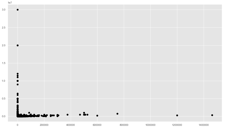
plt.scatter(Installment, Premium, c='black', s=50)
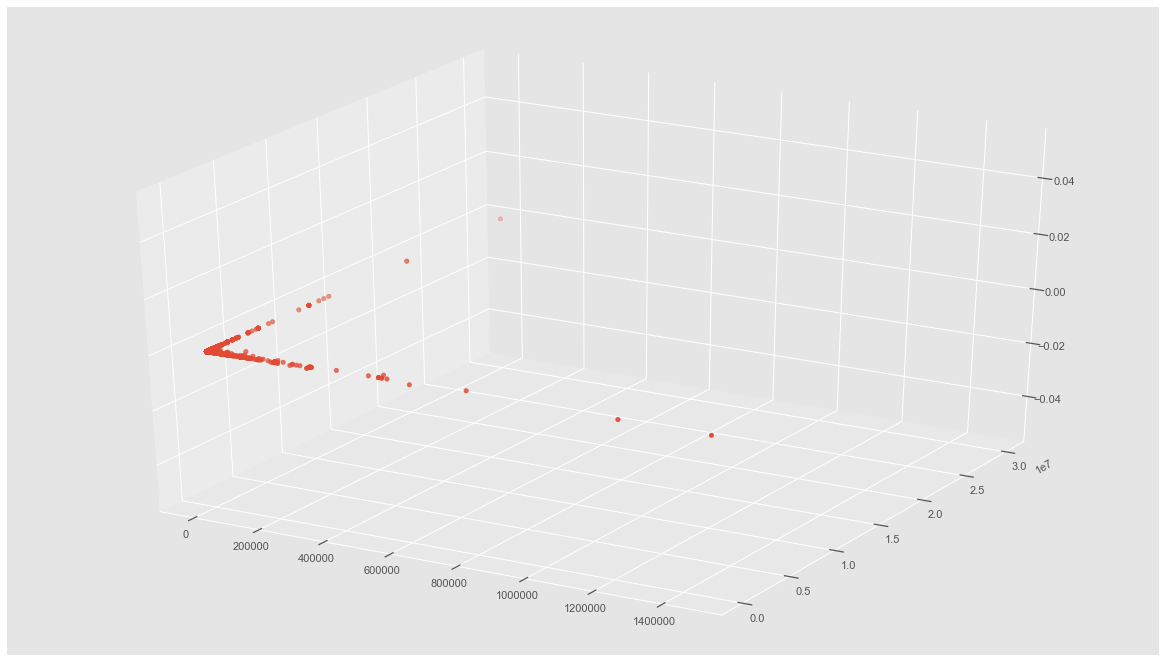
##plot in 3D space
from mpl_toolkits.mplot3d import Axes3D

fig = plt.figure()
ax = Axes3D(fig)
ax.scatter(X[:, 0], X[:, 1])
dataset = data.iloc[:,[16,18]]
X=dataset.iloc[:,[0,1]].values
X
array([[1463119,  329954],
       [1200000,  300000],
       [ 750000,  750000],
       ...,
       [      0,   50000],
       [      0,   30900],
       [      0,   30675]], dtype=int64)
#Using the elbow method to find the ideal number of clusters
from sklearn.cluster import KMeans
wcss = []
for i in range(1,11):
    km=KMeans(n_clusters=i,init='k-means++', max_iter=300, n_init=10, random_state=0)
    km.fit(X)
    wcss.append(km.inertia_)
plt.plot(range(1,11),wcss)
plt.title('Elbow Method')
plt.xlabel('Number of clusters')
plt.ylabel('wcss')
plt.show()
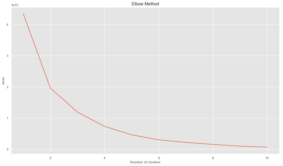
Ideal K size = 4,5,6
#Calculating the silhoutte coefficient
from sklearn.metrics import silhouette_score
from sklearn.cluster import KMeans


for n_cluster in range(2, 11):
    kmeans = KMeans(n_clusters=n_cluster).fit(X)
    label = kmeans.labels_
    sil_coeff = silhouette_score(X, label, metric='euclidean')
    print("For n_clusters={}, The Silhouette Coefficient is {}".format(n_cluster, sil_coeff))
For n_clusters=2, The Silhouette Coefficient is 0.9934664851024786
For n_clusters=3, The Silhouette Coefficient is 0.9482019450001424
For n_clusters=4, The Silhouette Coefficient is 0.9403171140499658
For n_clusters=5, The Silhouette Coefficient is 0.903696294345598
For n_clusters=6, The Silhouette Coefficient is 0.8209100056819879
For n_clusters=7, The Silhouette Coefficient is 0.8209194931504735
For n_clusters=8, The Silhouette Coefficient is 0.8205152286640742
For n_clusters=9, The Silhouette Coefficient is 0.740046045775413
For n_clusters=10, The Silhouette Coefficient is 0.7469443387160237
import pylab as pl
from sklearn.decomposition import PCA

Nc = range(1, 20)
kmeans = [KMeans(n_clusters=i) for i in Nc]
kmeans
score = [kmeans[i].fit(X).score(X) for i in range(len(kmeans))]
score
pl.plot(Nc,score)
pl.xlabel('Number of Clusters')
pl.ylabel('Score')
pl.title('Elbow Curve')
pl.show()

print(score)
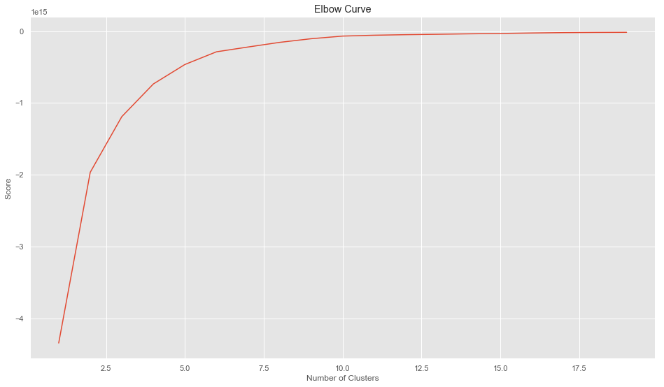
[-4342885204296660.0, -1965246538483911.8, -1190849308786024.8, -735865989905271.1, -464847169949274.5, -288260660074600.3, -221593993407933.6, -157027108634278.66, -106136302511251.6, -69345722080836.19, -57571566408134.14, -49745133662816.21, -44210314228213.82, -37851157457083.914, -32932468783416.984, -26461974880429.766, -21260906227471.258, -18700418224852.87, -17319322252699.422]
##Fitting kmeans to the dataset
km4=KMeans(n_clusters=4,init='k-means++', max_iter=300, n_init=10, random_state=0)
y_means = km4.fit_predict(X)
#Visualising the clusters for k=4
plt.scatter(X[y_means==0,0],X[y_means==0,1],s=50, c='purple',label='Cluster1')
plt.scatter(X[y_means==1,0],X[y_means==1,1],s=50, c='blue',label='Cluster2')
plt.scatter(X[y_means==2,0],X[y_means==2,1],s=50, c='green',label='Cluster3')
plt.scatter(X[y_means==3,0],X[y_means==3,1],s=50, c='cyan',label='Cluster4')

plt.scatter(km4.cluster_centers_[:,0], km4.cluster_centers_[:,1],s=200,marker='s', c='red', alpha=0.7, label='Centroids')
plt.title('Customer segments')
plt.xlabel('Installments')
plt.ylabel('Premium')
plt.legend()
plt.show()
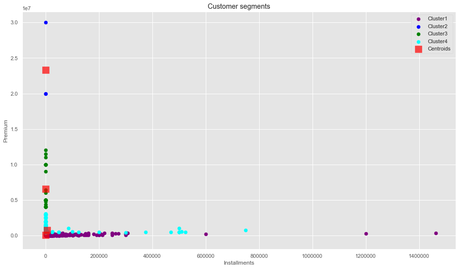
K- Means clustering didn’t turn out to be effective due to problems with the data collection procedure and poor data Quality
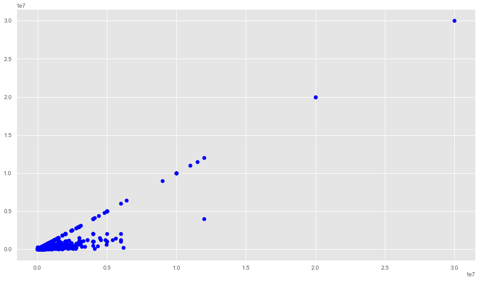
Identifying Patterns And Relationships
TP = data['Total.Paid'].values
Premium = data['Premium_Amount'].values
M = np.array(list(zip(TP, Premium)))
plt.scatter(TP, Premium, c='blue', s=50)
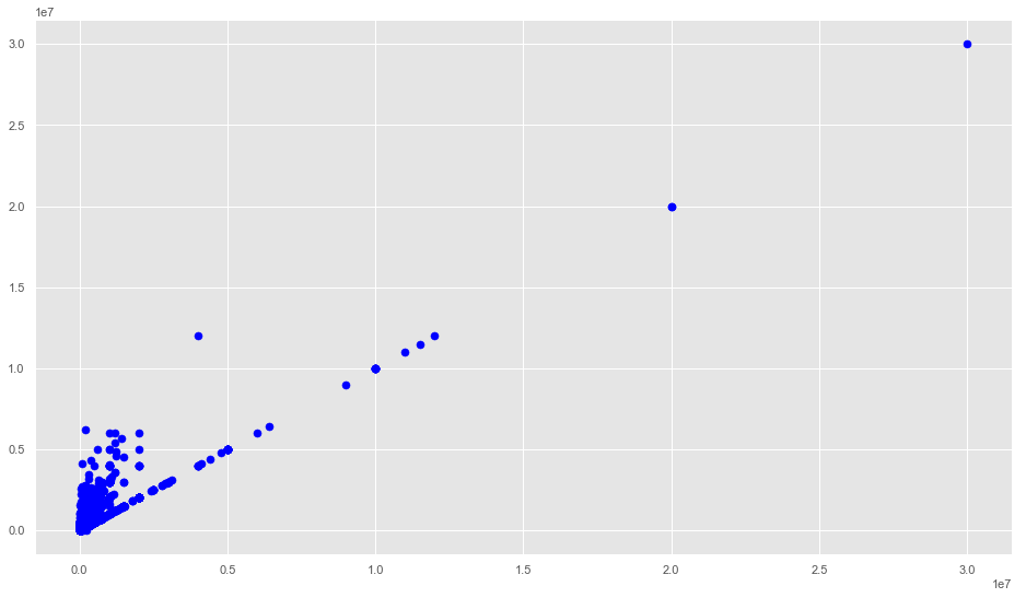
TP = data['Premium_Amount'].values
Premium = data['Total.Paid'].values
M = np.array(list(zip(TP, Premium)))
plt.scatter(TP, Premium, c='blue', s=50)
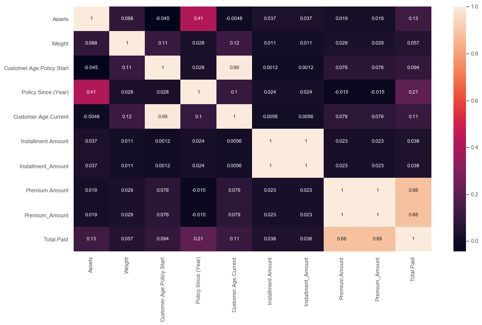
Identifying Important Correlations
sns.heatmap(data.corr(),annot=True)
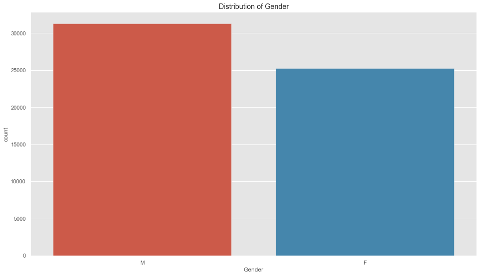
sns.countplot(x='Gender', data=data);
plt.title('Distribution of Gender');
data.hist('Customer.Age.Policy.Start', bins=35,);
plt.title('Distribution of Age');
plt.xlabel('Age');
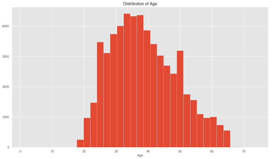
data['Customer.Age.Policy.Start'].mean()
38.890749023282126
The Average age tend to be around 39, and there are more Males in this Dataset than Females
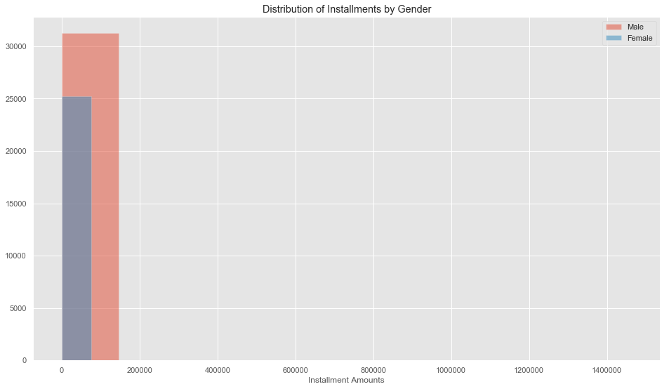
plt.hist('Installment_Amount', data=data[data['Gender'] == 'M'], alpha=0.5, label='Male');
plt.hist('Installment_Amount', data=data[data['Gender'] == 'F'], alpha=0.5, label='Female');
plt.title('Distribution of Installments by Gender');
plt.xlabel('Installment Amounts');
plt.legend();
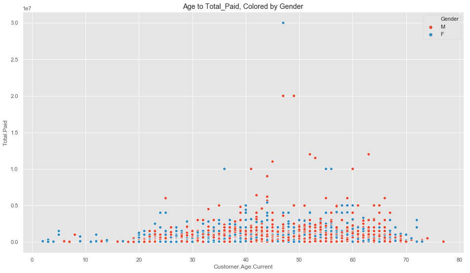
sns.scatterplot('Customer.Age.Current', 'Total.Paid', hue='Gender', data=data);
plt.title('Age to Total_Paid, Colored by Gender');